Journey into the Zone (Plates)

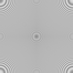
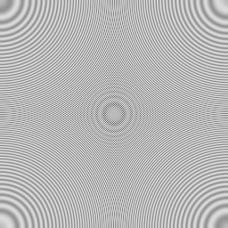
I have experimented recently with zone plates, which are the 2‑D equivalent of a chirp. Zone plates make for excellent test images to detect deficiencies in image processing algorithms or display and camera calibration. They have interesting properties: Each point on a zone plate corresponds to a unique instantaneous wave vector, and also like a gaussian a zone plate is its own Fourier transform. A quick image search (google, bing) turns up many results, but I found all of them more or less unusable, so I made my own.

Zone Plates Done Right

I made the following two 256×256 zone plates, which I am releasing into the public so they can be used by anyone freely.

Cosine zone plate

Sine zone plate

On both images, I shifted the origin of the wave function to the lower left corner so that the high frequencies, where usually the action is, appear in the center. The pixel values were calculated as

$I = 255 \left( { a y + 1 \over 2} \right) ^ {{}^1/_{\gamma}},$

where $I$ is the pixel value, $y$ is the wave function, $a$ is a contrast weighting function and $gamma$ is the display gamma exponent. The contrast weighting function is intended to correct for the effect of box shaped pixels (more about that below). The gamma exponent corrects for the non-linear sRGB transfer curve, and is chosen so that 50% grey corresponds to a pixel value of 187.

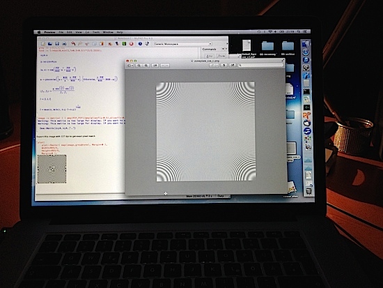
It is possible that your browser messes with these images and your don’t get to see them as they were intended. You can right click on these images and select “Save image to Downloads...” to get the verbatim version. To give you an impression how it should look like, here is a photo taken from my Mac with the cosine zone plate opened in the Preview application, at 2× zoom (on a retina display, the effective zoom factor was 4). The average grey value of the entire zone plate should be uniform, without any Moiré patterns, and all rings should appear to have the same contrast between them:

The Wave Function

The wave function $y$ is one of

$\begin{align*} y &= \cos \pi R ( u^2 + v^2 ) & \text{or} & & y &= \sin \pi R ( u^2 + v^2 ), \end{align*}$

depending on whether the cosine or the sine version is desired. The image coordinates $u$ and $v$ are assumed to be in the range 0…1 with the origin in the lower left corner. The resolution parameter $R$ is equal to the image dimension in pixels (which is 256 here).

The Apparent Wave Vector

The instantaneous wave vector $\vec{k}$ can be found by analyzing how fast the argument to the cosine or sine function changes per pixel when either $u$ or $v$ changes. It becomes

$\vec{k} = \begin{pmatrix} k_u \\ k_v \end{pmatrix} = \pi \frac{R}{R} \begin{pmatrix}\tfrac{\partial}{\partial u} \\ \tfrac{\partial}{\partial v} \end{pmatrix} ( u^2 + v^2 ) = 2 \pi \begin{pmatrix} u \\ v \end{pmatrix} ,$

where the elements $k_u$ and $k_v$ are the spatial frequencies along $u$ and $v$ direction, in radians per pixel. Each component hits the Nyquist limit when it reaches $\pi$ radians per pixel (equal to a wavelength of 2 pixels), which happens halfway along each coordinate. Beyond this limit the frequency folds back giving a mirror copy. The apparent wave vector $\vec{k}'$ that takes into account this frequency folding is

$\vec{k}' = 2 \pi \begin{pmatrix} \min u, 1 - u \\ \min v, 1 - v \end{pmatrix} .$

The Contrast Weighting Function

Now I’m going to explain the contrast weighting function $a$ , which is

$a = \frac{4}{ \pi^2 \, \operatorname{sinc} \frac{k'_u}{2} \, \operatorname{sinc} \frac{k'_v}{2} } .$

where $\operatorname{sinc} \, x = {\sin x \over x}$ is the unnormalized cardinal sine function. This is the inverse transfer function of a 1 by 1 pixel wide box filter, normalized to unity. To understand why this additional function is employed, I’m going to discuss an idealized mathematical model of a computer display.

A computer screen with perfectly “box shaped” pixels can be modeled mathematically as sequence of two transformations, as shown in the figure above. On the left is the original continuous signal, as it is computed by our wave function. In a first step this signal is thought to be ring modulated with an “impulse lattice” to give the signal in the middle. This step is non-linear and is responsible for all the sampling artifacts, because it creates side bands. Finally, in a second step, the signal is convolved with a box filter to arrive at the pixellated end result on the right.

It is this box filter convolution of the last step that the weighting function $a$ seeks to neutralize. Without this correction, the pixellated signal would underrepresent the contrast of higher spatial frequencies. You can verify this effect for yourself by eyeballing the above figure from a distance or looking at a the filtered version below.

Conclusion: Should we do blur-correction like we do gamma-correction?

The theory behind the “contrast weighting function” suggests that this loss of contrast applies to all synthetically generated images. It would therefore be theoretically justified to employ some kind of sharpening post filter in a 3‑D engine together with a corresponding blurring of the source textures, on similar grounds as gamma correction: the texture artist working by visual feedback on a computer screen is likely to oversharpen the texture because the computer monitor does not faithfully reproduce the light field that should correspond to the texture 2‑D signal.

The Tenth Planet

If it existed