It is good to see how physically based shading is finally gaining momentum in real time graphics and games. This is something I have been advocating for a long time. Developers are spreading the word. I was especially surprised to learn about Call of Duty: Black Ops joining the club [1]. Even a slick 60 Hz shooter with no cycles to spare can afford to do PBS today!
This leads me to the topic of this post, the normalization of the Blinn-Phong specular highlight. Why am I writing about it? It came to my mind recently with the current batch of publications from people adopting physically based shading models. This got me checking the maths again and I compiled a list with normalization factors for different shading models, given here in this post. I would also like to elaborate a little on the model that I wrote about in ShaderX7 [2]. Be aware this post is a large brain dump.
Blinn-Phong Normalization: A paradigm shift for texturing
Let me first devote some lines to emphasize how this normalization business is not only a matter for engine developers or shader authors, but also for texture artist education.
Normalization means, in simple terms, that the shading model scales the intensity of the specular highlight in proportion to its angular size, such that the total reflected energy remains constant with varying surface smoothness, aka. glossiness. This may sound like a minor technical detail, but it really is a paradigm shift.
| standard blinn-phong | normalized blinn-phong |
|---|---|
| Specular map has all the details | Gloss map has all the details |
| Glossiness constant | Specular level constant (almost) |
With standard Blinn-Phong shading, artists were used to paint surface variation into a texture connected to specular/reflective intensity, while the glossiness was only an afterthought, often not textured at all. With a normalized shading model, all the detail goes into the glossiness texture, while it is the specular intensity that becomes boring. So, is everything different now? In short, yes. And to drive the point home, I’ll give a visual example.
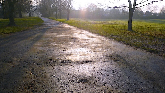
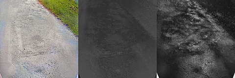
Consider the scene in the image above. The scene shows an an asphalt surface in backlight with dramatically different reflectances for wet and dry parts. Isn’t this paradox? The refractive index of water is actually lower than that of the asphalt minerals, so everything else being equal, the water-covered surface should have less reflection. But things are not equal, because the water-covered parts have a much smoother surface. A smoother surface focuses the reflected sunlight into a narrower range of outgoing directions, making it more intense at the same time. This is the reason for the glaring parts of the photo.
With this said, I dabbled a little bit with GIMP to try and factor the above image into diffuse, specular and glossiness textures, much in the same way as I had advised artists to do when I was technical director at Replay Studios. The result is shown below.
The diffuse texture is a straightforward idealization of the subsurface color, devoid of any lighting and reflections. Since this cannot be observed directly, it must be inferred, but it should be much more saturated than the real-world appearance. I may be useful to have photos taken with a polarizing filter as a reference.
The specular texture defines the reflectivity for the case when light, viewer and normal are aligned. This is the minimum value, and the shading model will increase the reflectivity for any other configuration. There is not much artistic freedom here, since this value is connected to refractive index of the material. It is usually in the range of 2% to 5% for everything which is not a metal or a crystal. In the example above, there is almost no point in texturing it.
Instead, all the surface variation went into the glossiness map. This map is taken to be a logarithmic encoding of the Blinn-Phong specular exponent, which is a measure of surface smoothness. Black represents a single-digit exponent, indicating a very rough surface. White represents an exponent in the thousands, indicating a very smooth surface. Since the shading model is normalized, both the size and the intensity of the specular highlight is controlled with this value alone.
| Texture | Physical interpretation |
|---|---|
| Diffuse | Color due to average subsurface absorption |
| Specular | Fresnel reflectance at normal incidence |
| Gloss | Blinn-Phong exponent, a measure of surface smoothness |
There is more to physically-based shading then just a normalized Blinn-Phong specular term. To get a dramatic and convincing contre-jour effect, it is important to model the behavior at grazing angles. This was one of the visual goals for the Velvet Assassin engine. See it realized, for example, in this scene, and also pay attention to the wet puddles on the floor, which is an effect of varying glossiness. Another play of varying glossiness are the wet streaks on the fuel tank here, or the dusty vs non-dusty parts on the car’s windscreen here. What’s more, it becomes possible to paint both metallic and non-metallic parts onto the same texture, which helps to minimize batch count and number of shader variants. (Edit 2018: The old youtube links were dead, so I replaced them with equivalent scenes from other videos.) As it turned out during the development, the Fresnel factor alone does not have enough ‘omph’. It needed the combination of a Fresnel factor and the micro-facet geometric visibility factor to get the right effect at grazing angles. More on this below.
In the earlier engine for SpellForce 2, there was only one material with a per-pixel varying glossiness like that, the ice/crystal material. It is possible to get a hint of how it looked like here and here (note how not only the specular highlight , but also the mipmap level of the translucent back buffer is varied depending on glossiness). Since this game was based on shader model 2, I needed to sacrifice shadow map taps to get the Blinn-Phong normalization in (without Fresnel). For all other materials, the glossiness was fixed and the normalization factor was a precomputed constant. What the engine did have was diffuse and specular hemisphere lighting. This allowed the artists to leave the diffuse texture black for parts of shiny metal, which is another important aspect of PBS. The soldier’s armor in this scene is a good example of reflecting sky- and ground colors. After some time, even these relatively crude, “physically inspired” shading models proved to be really popular with the team.
Normalization vs Energy Conservation
When I speak about normalization I understand a different thing than energy conservation. In energy conservation, one looks at the total hemispherical reflectance for a given BRDF, and guarantees that it is strictly bounded by unity for all incoming light directions. Normalization, on the other hand, is just as strong as we define it. We can demand, for instance, that some parameter (the specular exponent in this case) has no effect the total hemispherical reflectance for a single, conveniently chosen incoming light direction. Then we have normalized it. In mathematical terms,
![]()
It is possible (and may be even useful) to normalize BRDFs that are not energy conserving [8], like the original Phong and Blinn-Phong (the ones without the additional cosine term). It is also entirely possible to normalize something else than hemispherical reflectance, for instance we can normalize the micro-facet distribution function.
The Normalization Zoo
I verified the following list of normalization factors with the help of MuPAD, which is a great symbolic algebra tool. Unfortunately this is no longer available as a separate product, which is a real pity. I rate it second maybe only to Mathematica.
| Model | RDF/Integrand | Normalization | Literature |
|---|---|---|---|
| Phong | |||
| Phong (modified) |
[3,5,8] | ||
| Blinn-Phong | [6] | ||
| Blinn-Phong (modified) |
[3,9] | ||
| Model | NDF/Integrand | Normalization | Literature |
| Blinn-Phong (NDF) |
[2,4,5] | ||
| Blinn-Phong (heightfield) |
[10,11] |
The upper part of the table shows the normalized reflection density function (RDF). This is the probability density that a photon from the incoming direction is reflected to the outgoing direction, and is the BRDF times ![]() . Here,
. Here, ![]() is the angle between
is the angle between ![]() and
and ![]() , which is, for the assumed view position, also the angle between
, which is, for the assumed view position, also the angle between ![]() and
and ![]() , resp.
, resp. ![]() and
and ![]() . The literature column shows where I have seen these normalizations mentioned previously.
. The literature column shows where I have seen these normalizations mentioned previously.
The lower part of the table shows the normalized normal distribution function (NDF) for a micro-facet model. This is the probability density that the normal of a micro-facet is oriented towards ![]() . It is the same expression in spherical coordinates than that for of the Phong RDF, just over a different variable,
. It is the same expression in spherical coordinates than that for of the Phong RDF, just over a different variable, ![]() , the angle between
, the angle between ![]() and
and ![]() . The heightfield distribution does it slightly different, it normalizes the projected area of the micro-facets to the area of the ground plane (adding yet another cosine term).
. The heightfield distribution does it slightly different, it normalizes the projected area of the micro-facets to the area of the ground plane (adding yet another cosine term).
Two Pi Or Not Two Pi
This is a good opportunity to elaborate on this ![]() -business, because it can be confusing time and again. The RDFs and NDFs necessarily contain
-business, because it can be confusing time and again. The RDFs and NDFs necessarily contain ![]() , as the result of an integration over parts of a sphere. In the shader code however,
, as the result of an integration over parts of a sphere. In the shader code however, ![]() does usually not appear, because it cancels out when multiplying with irradiance, which is itself an integration over parts of a sphere.
does usually not appear, because it cancels out when multiplying with irradiance, which is itself an integration over parts of a sphere.
Consider a point light source modeled as a small and very far away sphere, at distance ![]() . Let this sphere have radius
. Let this sphere have radius ![]() and a homogeneous emissive surface of radiance
and a homogeneous emissive surface of radiance ![]() . From the point of view of the receiving surface, the solid angle subtended by this sphere is a spherical cap, and so the irradiance integrates to
. From the point of view of the receiving surface, the solid angle subtended by this sphere is a spherical cap, and so the irradiance integrates to ![]() . So there you have
. So there you have ![]() in the formula for the irradiance of a point light, neatly canceling with the
in the formula for the irradiance of a point light, neatly canceling with the ![]() from the RDF resp. NDF. This exercise can be done with all other types of illumination, it should always remove the factor
from the RDF resp. NDF. This exercise can be done with all other types of illumination, it should always remove the factor ![]() . (See the comment section for an in-depth explanation.)
. (See the comment section for an in-depth explanation.)
Minimalist Cook-Torrance (ShaderX7 style)
I wrote earlier in this post how it was important to capture the effects at grazing angles. The original Cook-Torrance model [7] has expensive factors for the distribution of normals (![]() ), the Fresnel reflectance (
), the Fresnel reflectance (![]() ) and geometric occlusion of micro-facets (
) and geometric occlusion of micro-facets (![]() ). The normalized Blinn-Phong distribution can be used to greatly simplify
). The normalized Blinn-Phong distribution can be used to greatly simplify ![]() . A clever simplification for
. A clever simplification for ![]() was given by Kelemen and Szirmay-Kalos [4], by combining
was given by Kelemen and Szirmay-Kalos [4], by combining ![]() with the foreshortening terms in the denominator; it should then be called the geometric visibility factor
with the foreshortening terms in the denominator; it should then be called the geometric visibility factor ![]() . The Schlick approximation is good to simplify
. The Schlick approximation is good to simplify ![]() , but still with all the lerp’ing and one-minus’ing that is going on, it generates many shader instructions.
, but still with all the lerp’ing and one-minus’ing that is going on, it generates many shader instructions.
For Velvet Assassin, I devised a further approximation by combining the effect of ![]() and
and ![]() in a single expression with a significantly reduced instruction count, which I would call ‘minimalist Cook-Torrance’. I looked at graphs and found, that in order to capture the essence, it suffices to divide by a higher power of
in a single expression with a significantly reduced instruction count, which I would call ‘minimalist Cook-Torrance’. I looked at graphs and found, that in order to capture the essence, it suffices to divide by a higher power of ![]() , and get rid of
, and get rid of ![]() altogether. This is where the odd power of 3 comes from. In BRDF form, this is
altogether. This is where the odd power of 3 comes from. In BRDF form, this is
![]()
where ![]() is the diffuse reflectance,
is the diffuse reflectance, ![]() is the specular reflectance, and
is the specular reflectance, and ![]() is the specular exponent. This is the formula that was published in the ShaderX7 article [2] and the one that shipped with Velvet Assassin (see here for the code). The formula can be decomposed into a contribution from
is the specular exponent. This is the formula that was published in the ShaderX7 article [2] and the one that shipped with Velvet Assassin (see here for the code). The formula can be decomposed into a contribution from ![]() (the normalized Blinn-Phong NDF, see table above) and a contribution from the product of
(the normalized Blinn-Phong NDF, see table above) and a contribution from the product of ![]() and
and ![]() :
:
![]()
It is possibly the crudest approximation to Cook-Torrance there is, but an effective one no less. There will be no Fresnel color shift and no explicit interpolation to white (saturation is supposed to take care of that), so the model is linear in ![]() , which is a computational advantage of its own. The model will underestimate the reflectance at grazing angles for low-index materials like water, and overestimate the reflectance for high-index materials like metals. For the typical range of di-electrics however, the estimation is just right.
, which is a computational advantage of its own. The model will underestimate the reflectance at grazing angles for low-index materials like water, and overestimate the reflectance for high-index materials like metals. For the typical range of di-electrics however, the estimation is just right.
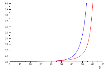
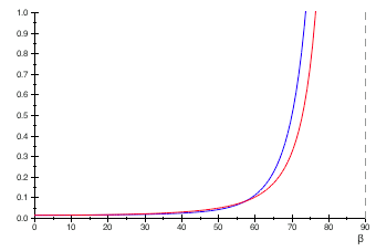
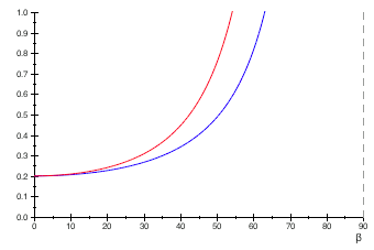
The graphs above show the minimalist model with the ![]() denominator (red graph) against the combined effect of Schlick and the
denominator (red graph) against the combined effect of Schlick and the ![]() denominator of Kelemen and Szirmay-Kalos (blue graph), for specular reflectances of 0.02 (top), 0.05 (middle) and 0.8 (bottom), respectively. The graphs do not align perfectly, but the ‘omph’ is there. So, what about the instruction count?
denominator of Kelemen and Szirmay-Kalos (blue graph), for specular reflectances of 0.02 (top), 0.05 (middle) and 0.8 (bottom), respectively. The graphs do not align perfectly, but the ‘omph’ is there. So, what about the instruction count?
| Minimalist | F‑Schlick with Kelemen/Szirmay-Kalos |
|---|---|
| Multiply denominator by |
Calculate |
| Raise that to the 4th or 5th power. | |
| Calculate |
|
| Lerp. |
If you already have ![]() , the simplified model just needs one additional multiplication. The combination of F‑Schlick and Kelemen/Szirmay-Kalos needs 5 or 6 more instructions in a dependency chain from that point. It doesn’t help if a Fresnel factor from the environment map already exists, since that is based on
, the simplified model just needs one additional multiplication. The combination of F‑Schlick and Kelemen/Szirmay-Kalos needs 5 or 6 more instructions in a dependency chain from that point. It doesn’t help if a Fresnel factor from the environment map already exists, since that is based on ![]() . In terms of bang for the buck, if there are many lights in a loop (and I had a forward renderer with up to 8 lights per pass), then I’d recommend the minimalist version.
. In terms of bang for the buck, if there are many lights in a loop (and I had a forward renderer with up to 8 lights per pass), then I’d recommend the minimalist version.
References
[1] Dimitar Lazarov, “Physically-based lighting in Call of Duty: Black Ops” SIGGRAPH 2011 http://advances.realtimerendering.com/s2011/index.html
[2] Christian Schüler, “An Efficient and Physically Plausible Real-Time Shading Model.” ShaderX 7, Chapter 2.5, pp. 175–187
[3] Fabian Giesen, “Phong Normalization Factor derivation” http://www.farbrausch.de/~fg/stuff/phong.pdf
[4] Kelemen and Szirmay-Kalos, “A Microfacet Based Coupled Specular-Matte BRDF Model with Importance Sampling”, Eurographics 2001 http://www.fsz.bme.hu/~szirmay/scook.pdf
[5] Lafortune and Willems, “Using the modified Phong reflectance model for physically based rendering”, Technical Report http://graphics.cs.kuleuven.be/publications/Phong/
[6] Yoshiharu Gotanda, “Practical Implementation of Physically-Based Shading Models at tri-Ace”, SIGGRAPH 2010
http://renderwonk.com/publications/s2010-shading-course/
[7] Robert Cook and Kenneth Torrance, “A reflectance model for computer graphics” http://citeseerx.ist.psu.edu/viewdoc/summary?doi=10.1.1.83.7263
[8] Robert Lewis, “Making Shaders More Physically Plausible”, Computer Graphics Forum, vol. 13, no. 2 (June, 1994)
http://users.tricity.wsu.edu/~bobl/personal/mypubs/1993_plausible.pdf
[9] Akienne-Möller, Haines and Hoffmann, “Real-Time Rendering” book
http://www.realtimerendering.com/
[10] Pharr, Humphreys, “Physically-Based Rendering” book
http://www.pbrt.org/
[11] Nathaniel Hoffmann, “Crafting Physically Motivated Shading Models for Game Development”, SIGGRAPH 2010
http://renderwonk.com/publications/s2010-shading-course/
Pingback: PBR 四 法线分布函数 - 算法网